This is the third post in a series that is exploring sketching techniques to count unique items. In the first post, I explored the HyperLogLog (HLL) data structure and its implementation in Redis. In the second post, I expanded on the topic of unions and intersections of sets using HyperLogLogs.
Regarding intersections, I showed how the Inclusion/Exclusion principle could be used to compute intersection cardinalities. However, in studies conducted by others, the method has been found to produce inaccurate results in some conditions.
In this post, I explore a different sketching technique that claims to improve the accuracy of these results. I also provide the results of tests I did comparing the accuracy of the two methods. Since I will be using terminology introduced in the last post, I request readers to familiarise themselves with those first before continuing here.
Intersection counts using the MinHash sketch
In my research to solve the problem of improving accuracy of intersection cardinalities, I found an effort by AdRoll who introduced a different approach to solve this problem using a new sketching method called k-MinHash.
The MinHash (MH) sketch is a way to estimate a quantity called the Jaccard coefficient of sets, which measures how similar two sets are. Mathematically, given two sets A and B, Jaccard coefficient is defined as | A n B | / | A u B |. So, MH(A, B) is approximately | A n B | / | A u B |. Hence,
| A n B | is approximately equal to MH(A, B) x | A u B |.
Note that we can compute | A u B | by merging individual HLLs, as unions are lossless.
The MinHash sketch
I found this blog to be an excellent introduction to MinHash, including a proof of how it approximates to the Jaccard coefficient. The MinHash sketch involves computing the hash of every element in the set, and maintaining k elements which have the smallest hashes from which the Jaccard coefficient is derived. Since k will be very small compared to the set’s cardinality in our cases, this is also a space-efficient sketching technique.
Understanding MinHash
The intuitive understanding for MinHash is as follows, summarised from the blog above:
- Define hmin(S) as the element with smallest hash in S.
- Given two sets A and B, if hmin(A) = hmin(B) (say, an element ‘x’), then it can be proved that x = hmin(A u B) and x is in A n B. This can be proved by contradiction. Say x is not in hmin(A u B), there must be an element ‘y’ = hmin(A u B) that has a smaller hash than x, but that element should have been either hmin(A) or hmin(B). Hence, by contradiction, x = hmin(A u B). Now, since hmin(A) = hmin(B), assuming a good hash function, x is in A & B, i.e. x is in A n B.
- If h is a good random hashing function, x can be assumed to be a random element in A u B.
- Probability(hmin(A) = hmin(B)) = Probability of a random element of A u B that is also present in A n B. The latter quantity is | A n B | / | A u B |, which is the Jaccard coefficient. So we see that the probability of an element with the smallest hash being in two sets can be linked to the Jaccard Coefficient.
To make this argument stronger and avoid a freak hashing function accident, we look for not 1, but k min values in the MinHash set that could belong to both A and B. I find this approach somewhat similar to how we used stochastic averaging in the HLL case. There seem to be two ways of getting k values. The first is to have k different hash functions and use the same element in the set. However, since it is going to be difficult to find so many good hashing functions, we instead use the same hash function and compare not 1 but k different elements in the two MinHash sets. The blog above describes how the proof can be extended to k values, and the way to compute the probabilities in such a case. I leave that out of this blog and the interested readers can get it from there.
Although the blog mentions a value of k as small as 400, in my experiments I have found good results only with k being 4096 or 8192 (which are closer to the numbers mentioned in the AdRoll blog).
MinHash Algorithm
The algorithm for computing MinHash is as follows:
Given 2 sets A & B, and a fixed ‘k':
- Define a hash function that maps A & B elements to hashed integer values.
- Define hmin(S, k) = elements of S with smallest k hashes.
- As elements are seen from A and B, maintain hmin(A, k) and hmin(B, k) by keeping the k smallest hashes in each set.
- Compute hmin(hmin(A, k) u hmin(B, k), k). This is the same as hmin(A u B, k). This can be deduced using similar logic to the proof shown above when k=1. Let hmin(A u B, k) = X
- Compute X n hmin(A, k) n hmin(B, k) = Y. These are elements with smallest hashes that belong to A u B and A n B.
- Jaccard coefficient (A, B) = approximately | Y | / k
Implementing the MinHash sketch using Redis
To implement the MinHash algorithm, we can use a state store that:
- can store a set of the actual items and their hash values together
- is able to sort these items on the hash values so as to maintain the smallest k values
- can intersect and merge these sets
As it happens, Redis has a very suitable data structure that supports these operations – the sorted set. Each MinHash structure can be a sorted set with the item as the member and the hash as its score on which Redis sorts and maintains the order of the set. This feels ideal because given the high throughput, low latency characteristics of Redis, we can use it as a shared state store and manage the MinHash sets as part of a streaming application.
Using a Redis sorted set, we can do the following:
- Add the first k items along with their hashes to the set, using ZADD
- From then, update the set by replacing the member with the highest rank with the incoming item provided the incoming item’s hash is smaller. ZRANGE and ZREM family of functions provide these capabilities.
- We can use ZUNIONSTORE and ZINTERSTORE to get the required intermediate sets X and Y mentioned above.
- ZCARD gets the cardinality of the sets required for computing the Jaccard coefficient.
Since my goal for the time being is to compare accuracy, I have not considered performance characteristics of this algorithm too much, and improvements could be possible.
Comparing Inclusion/Exclusion principle and MinHash for intersection accuracy
Test Setup
To evaluate how the two methods we have seen so far fare against each other in terms of accuracy, I used the same test design as what Neustar followed, that I spoke about in the last post, (although I have certainly not been as exhaustive as them). Specifically, the test parameters were driven by the two measures:
- overlap(A, B) = | A n B | / | B |, where B is the smaller set.
- cardinality_ratio(A, B) = | A | / | B |, where B is the smaller set.
I kept the value of | B | fixed and then varied | A | and | A n B |. Once the cardinalities of A, B and A n B were decided, I generated random numbers between 1 and 1B such that the required cardinality constraints were met. For each combination of A, B and A n B, I generated 100 such sets and ran the tests. The results were averaged over the 100 tests. Each run for one such combination of A, B and A n B did the following:
- Added elements of A and B to respective HyperLogLog keys in Redis
- Added elements of A and B to respective MinHash keys (backed by Redis sorted sets as described above)
- Computed A n B using HLLs and the Inclusion / Exclusion method.
- Computed A n B using KMinHash
The results for each run were logged, then compared for accuracy.
Remember that there were thresholds for overlap and cardinality within which Neustar found Inclusion/Exclusion to be satisfactory. I divided the test data into two categories – one which satisfied the thresholds (the good case) and one which didn’t (the bad case). For the HLL register size in Redis, the good case was when:
- overlap(A, B) >= 0.05, AND
- cardinality_ratio(A, B) < 20
For the good case, I fixed | B | as 10000, and created values for | A | and | A n B | that satisfied the above criteria. So for e.g. I took values of 0.05, 0.1, 0.2, 0.5, 0.75 for overlap. This gives the required | A n B | values. Similarly, I took values of 2, 5, 10 and 17.5 for cardinality ratio. This gives the required values for | A |.
For the bad case, I fixed | B | as 1000 (a smaller value). The values for B and | A n B | were created such that they violated either both the criteria or just the cardinality_ratio. I was motivated by a use case where one of the sets was very small compared to the other. Remember a use case where a publisher may be looking to see which people from a particular locality visit a particular web page. In this, the number of users visiting a popular web page would be very large, but the number of people in a locality could get very small.
Given | A |, | B | and | A n B |, I ran the tests for all combinations of these. In each case, I computed the % error of | A n B | when computed using both Inclusion / Exclusion and KMinHash.
Test Results
The results below are aggregated and averaged by cardinality ratio and overlap individually. For example, when averaged by cardinality ratio, it computes the average of error percentages across all chosen overlap values.
The following are the results from the runs with good threshold parameters:
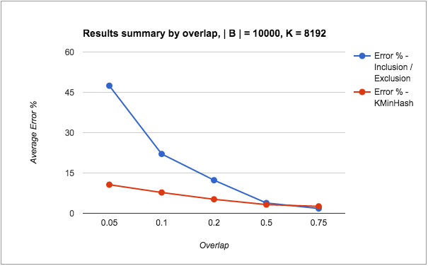
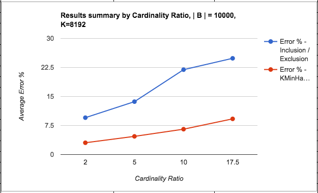
The following points can be made from the results:
- The error % of intersection counts through both methods seem to be significantly higher than the erro % of HLLs itself, irrespective of the sketching method used. Not shown here, but observed in my tests is that the error % of the individual HLLs are always quite small – < 0.5%.
- The accuracy of both KMinHash and Inclusion/Exclusion improves as the overlap increases (i.e. the intersection count is larger than any individual error terms) or when cardinality ratio decreases (i.e. the set sizes are comparable to each other, thereby one set doesn’t contribute a huge error term compared to the intersection count). This is as expected.
- KMinHash performs better than Inclusion / Exclusion for almost all cases except where the overlap is quite high, when Inclusion / Exclusion seems to be marginally better.
- KMinHash errors seem to be more linear in nature compared to Inclusion/Exclusion errors.
The following are the test results from runs with bad threshold parameters:
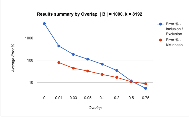
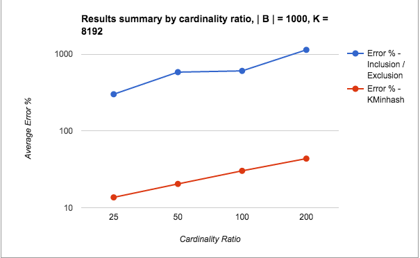
Note: The scale for the y-axis is switched to log scale for showing the results clearly.
The following points can be made from the test results:
- The error percentages for the pathological cases is quite bad for Inclusion / Exclusion (in the order of 1000s), whereas KMinHash seems to be performing quite a lot better.
- Even otherwise, KMinHash is performing significantly better than Inclusion / Exclusion in most cases.
- As seen for the good cases, with increasing overlap and decreasing cardinality ratio, the error percentages improve as usual.
- The really bad performance of the Inclusion Exclusion method for low overlaps (very small A n B) when taken in context may not appear substantially bad.We are talking about intersection counts of 50 and less sometimes and it may not be too bad to just predict these as 0. However, what is interesting to note is the KMinHash is able to perform better even for such very small cases and predict good values.
- Values of overlap higher than 0.05 are within threshold limits for the overlap, however values of the cardinality ratio are outside of the threshold limits. The results show that the error values are high even when one of the two measures is outside the threshold values.
- Again, high overlap cases seem to perform well in Inclusion / Exclusion compared to KMinHash, although again, the difference is marginal.
- Another point not shown here is that the standard deviation of the error percentages for KMinHash is much lesser than Inclusion / Exclusion method in all cases – thereby indicating more reliable performance.
Conclusion
In conclusion, we can say that getting intersection counts through sketching techniques do carry a reasonable error percentage that needs to be considered when exposing analytics using them. KMinHash is an effective sketching technique that gives more accurate results for intersection counts compared to the Inclusion/Exclusion method of HLLs. The method I have discussed here is probably not as space or time efficient as the HLL Inclusion/Exclusion method. So, as of now, it is a tradeoff between accuracy and performance characteristics that should be considered when picking an implementation. In a future post, I will try and discuss the performance characteristics of the KMinHash method in more detail.
Pingback: Counting unique items fast – Better inter...