Tag Archives: sketching

Redis HyperLogLog and KMinHash performance

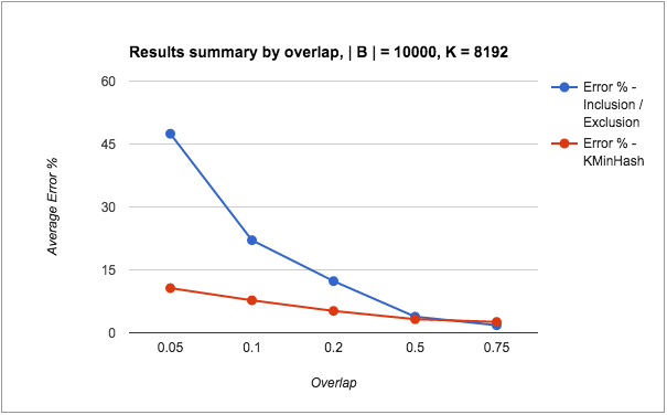
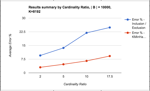
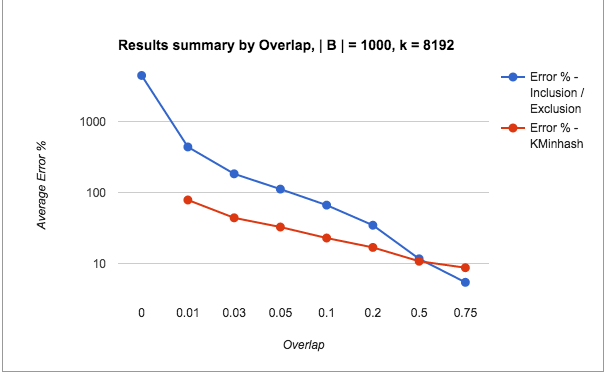
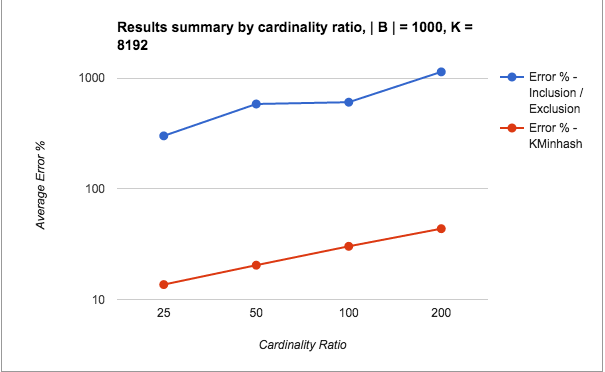
The last few blog posts explored the topic of counting unique items efficiently using two specific sketching techniques – HyperLogLogs (HLLs) and KMinHash. The underlying motivation of these techniques was to use probabilistic data structures for counting high cardinality data sets, with a focus on being efficient in both time and space, trading off some accuracy in the counts. For high cardinality data sets, this is a reasonable tradeoff in some domains. We saw how HLLs in Redis provided unique counts with an error of about 0.18% with a bounded 12KB memory size per key. We also saw how well additional operations like unions and intersections fared with HLLs, and how KMinHash provided a more accurate measure over HLLs for intersection operations.

One of the strong advantages of sketching techniques is their efficiency vis-a-vis time and space system measures. Therefore, while we concluded that KMinHash provided more accurate results over HLLs for intersections, it would be good to set it in context alongside a performance comparison so that tradeoffs can be made between accuracy and performance. The purpose of this blog post is to cover the system performance measures of the two methods, using Redis as a store for the counts.

Context for the performance tests

All tests involved two sets: Set A: 175,000 elements, Set B: 10,000 elements, and their intersection Set A n B: 7,500 elements. The elements were added to Redis data structures using Python client code.

The test code operated in two phases. The first added the elements to keys representing the HLL and KMinHash sets. Once all additions were completed, the second phase computed the intersection cardinality using HLL Inclusion/Exclusion principle and the KMinHash method, respectively. The details of the HLL based implementation have been covered in the first and second posts. The KMinHash algorithm has been covered in the third post. Readers can review those posts to familiarise themselves with the details.

The tests were performed on a MacBook Pro 1.6 GHz Intel Core i5 processor, 4 GB 1600 MHz DDR3 RAM. Redis version was 3.0.3 compiled from source, and started with default configuration (at least, as far as the performance related configuration goes). The test code used Python Redis client 2.10.3.

Implementation details

Counting with HLLs

For HLLs, the add phase used PFADD with Redis pipeline mechanism, and a pipeline batch size of 10,000. The compute phase merged the HLL keys using PFMERGE to compute A u B and then computed the intersection count using the Inclusion/Exclusion principle.

Here’s how the add phase looks like:

Counting with KMinHash

For KMinHash, recall that the algorithm was implemented using Redis sorted sets storing the IDs as items in the set sorted according to their hashes (which acted as scores). The add phase added/updated elements in the Redis sorted sets. The compute phase computed the Jaccard coefficient estimate using the algorithm described in post 3, and from there computed A n B cardinality.

At the time of computing the Jaccard coefficient, we should only consider the ‘k’ minimum values of the MinHash sets. However, the sets may have more than ‘k’ elements during the add phase. This gives us a knob to tradeoff between time and memory. For example, we could either keep exactly ‘k’ elements at all times thereby making sure that memory is bounded. This does require more operations in the add phase to ensure the cardinality is maintained (via a ZREM operation, for instance). The motivation to keep the memory bounded might come if we need to maintain a lot of such MinHash sets (say, for different dimensions being measured) and cumulatively, the amount of memory might shoot up very high. On the other hand, we could allow the memory to be slightly unbounded, but make the add operation very fast. This could be a valid strategy if the number of additions is going to happen very fast and saving on time is crucial.

Based on the above choices, I tried three different approaches for implementing KMinHash.

  • Optimise for time (time-optimised): Add multiple elements as a batch using the Redis pipeline mechanism, and truncate the batch to the size of ‘k’ once we have added the batch. Note that in this approach, the MinHash set’s size could grow beyond ‘k’ (depending on the size of the batch).

Here’s how the add phase looks using batch addition. Note the cardinality adjustment at the end of the batch.

  • Optimise for memory (mem-optimised): Bound the cardinality of the KMinHash sets to ‘k’ at add time itself. We do this by truncating the MinHash set to ‘k’ elements after any addition that potentially increases the set’s size. We maintain some state on the client – the current cardinality of the sorted set and the current max MinHash value. This state acts as a cache to help avoid some calls to the Redis server.

This is how the mem-optimised version looks. Note the cardinality adjustment after every add post ‘k’ elements. The local state is maintained in variables like elements_added and max_min_hash

  • Server side scripting (scripting): Redis has a mechanism to execute something akin to stored procedures of a database, by writing them using the LUA scripting language. In this method, define a LUA script that updates the KMinHash set keeping the cardinality bounded to ‘k’. Call this script in pipeline mode during the add phase using the Redis command EVAL or EVALSHA.

Here’s the Lua script that is loaded and executed in the Redis server process. Note how the cardinality is adjusted after every addition post ‘k’ elements. The difference with the mem-optimised approach is that all state is maintained in Redis itself.

The native support for HLL in Redis acts as an advantage and it should be intuitively clear that HLLs score better than KMinHash overall. So, this is not really to show whether KMinHash is better than HLL (which it is not), but to illustrate the comparative system measures for similar cardinality sets in both approaches, as also among the various KMinHash implementation strategies.

Time comparison

Things to measure here included the time indicators between HLL and KMinHash implementations, and also across the various KMinHash implementations. To compare various KMinHash implementations, the high level ‘time’ command was used. The tests were run multiple times to see stability of the time measures across different data sets. The results of the same are as below:

  • KMinHash – time-optimised: 8.5 seconds (average real time)
  • KMinHash – mem-optimised: 13.85 seconds (average real time)
  • KMinHash – scripting: 11.2 seconds (average real time)

Note that this time includes the add phase and compute phase; however, since the HLL addition and cardinality computation is fixed, the time difference is only accounted for by the various KMinHash strategies used.

To compare times between HLL and KMinHash specifically, the Python profiler cProfile was used and the cumulative time measured across individual calls. The results are as below:

  • HLL addition: 6.1 seconds
  • KMinHash addition – time-optimised: 7.2 seconds
  • KMinHash addition – mem-optimised: 12.9 seconds
  • KMinHash addition – scripting: 10.2 seconds
  • HLL intersection: 0
  • KMinHash intersection – time-optimised: 0.03 seconds
  • KMinHash intersection – mem-optimised: 0.04 seconds
  • KMinHash intersection – scripting: 0.02 seconds

Note that the times in the profiled runs don’t add up exactly to the measurements using the ‘time’ command. I suspect this could be due to the profiler overhead.

From the above, we can draw the following conclusions:

  • As expected, HLL performance is the best among all approaches in terms of time measures.
  • The best performance among KMinHash approaches is from the time-optimised approach, followed by the Lua scripting approach and finally by the mem-optimised approach. This is as expected.
  • The time-optimised approach is slower than the HLL approach by about 18%. In comparison, the slowest KMinHash approach (mem-optimised) is almost 100% slower.
  • The time difference for intersection computation is not significant to consider and hence additions is what should be considered for selecting an approach.

Memory comparison

In terms of memory, HLL is a very efficient data structure compared to sorted sets. There are probably parameters that can be tuned for optimising set memory as well, but these will likely cause some increased load on processing time. I did not consider this in my tests.

One thing to note is that the memory is bounded in both cases after the addition of all elements: 12KB for HLL, memory for max ‘k’ elements in KMinHash. The length of the objects used can be determined using the redis command DEBUG OBJECT <key-name>. The results after adding elements from a representative dataset to both HLL and KMinHash keys are as follows:

  • HLL key 175000 size: Serialized length 10491 bytes
  • HLL Key 10000 size: Serialized length 8526 bytes
  • KMinHash key 1 size: Serialized length 187530 bytes
  • KMinHash key 2 size: Serialised length 179048 bytes

One other thing that is relevant is how the memory grows as elements are added to the sets, as these spikes can cause pressure on Redis server memory when there are a lot of such sets. Referring to the various approaches for KMinHash, we see that the time-optimised approach can add more than ‘k’ elements as they are added in batches. To measure this, I ran the redis command INFO periodically and monitored the used_memory_peak_human value as the add phase was in progress. The results are as follows:

  • KMinHash – time-optimised: 67.2 MB
  • KMinHash – mem-optimised: 62.2 MB
  • KMinHash – scripting: 62.1 MB

With the Lua scripting technique, there is also an increase in the Lua memory used by Redis (used_memory_lua) to about 50176 bytes compared to the default of 36864 bytes.

My first implementation of the time-optimised technique adjusted the cardinality of the KMinHash set to ‘k’ only when the intersection cardinality was computed (sort of a lazy approach), instead of adjusting it after every batch addition. With this approach, the used_memory_peak_human value rose as high as 125.86 MB.

From the above, we can draw the following conclusions:

  • Memory used by KMinHash is an order of magnitude more than that used by HLL.
  • The mem-optimised approach is only marginally better in used_memory_peak compared to the time-optimised approach.
  • A lazy time-optimised approach that clears memory only at the end of the add phase does significantly increase memory consumption – almost 100% more than the optimised cases.

Conclusion

HLL is superior to KMinHash based implementations by a reasonable margin from a performance perspective, which is expected given that it is a highly optimised implementation in the Redis server. However, for the accuracy gains of KMinHash, the penalty doesn’t seem too high. Given that the time-optimised approach gives the best time performance, with only marginally weaker memory performance, it is possibly the best implementation overall for KMinHash. So, it could well be something that is implemented along side HLLs to provide an efficient and accurate unique value counting solution in a BigData analytics system.

While I have tried to optimise the code as much as I could, I might not have got everything completely right, as my Redis knowledge isn’t too high. If anyone has suggestions to improve this implementation, or alternate ideas, I request readers to please post those in comments for the benefit of all.

facebooktwittergoogle_plusredditpinterestlinkedinmail

Counting unique items fast – Better intersections with MinHash

This is the third post in a series that is exploring sketching techniques to count unique items. In the first post, I explored the HyperLogLog (HLL) data structure and its implementation in Redis. In the second post, I expanded on the topic of unions and intersections of sets using HyperLogLogs.

Regarding intersections, I showed how the Inclusion/Exclusion principle could be used to compute intersection cardinalities. However, in studies conducted by others, the method has been found to produce inaccurate results in some conditions.

In this post, I explore a different sketching technique that claims to improve the accuracy of these results. I also provide the results of tests I did comparing the accuracy of the two methods. Since I will be using terminology introduced in the last post, I request readers to familiarise themselves with those first before continuing here.

Intersection counts using the MinHash sketch

In my research to solve the problem of improving accuracy of intersection cardinalities, I found an effort by AdRoll who introduced a different approach to solve this problem using a new sketching method called k-MinHash.

The MinHash (MH) sketch is a way to estimate a quantity called the Jaccard coefficient of sets, which measures how similar two sets are. Mathematically, given two sets A and B, Jaccard coefficient is defined as | A n B | / | A u B |.  So, MH(A, B) is approximately | A n B | / | A u B |. Hence,

| A n B | is approximately equal to MH(A, B) x | A u B |.

Note that we can compute | A u B | by merging individual HLLs, as unions are lossless.

The MinHash sketch

I found this blog to be an excellent introduction to MinHash, including a proof of how it approximates to the Jaccard coefficient. The MinHash sketch involves computing the hash of every element in the set, and maintaining k elements which have the smallest hashes from which the Jaccard coefficient is derived. Since k will be very small compared to the set’s cardinality in our cases, this is also a space-efficient sketching technique.

Understanding MinHash

The intuitive understanding for MinHash is as follows, summarised from the blog above:

  • Define hmin(S) as the element with smallest hash in S.
  • Given two sets A and B, if hmin(A) = hmin(B) (say, an element ‘x’), then it can be proved that x = hmin(A u B) and x is in A n B. This can be proved by contradiction. Say x is not in hmin(A u B), there must be an element ‘y’ = hmin(A u B) that has a smaller hash than x, but that element should have been either hmin(A) or hmin(B). Hence, by contradiction, x = hmin(A u B). Now, since hmin(A) = hmin(B), assuming a good hash function, x is in A & B, i.e. x is in A n B.
  • If h is a good random hashing function, x can be assumed to be a random element in A u B.
  • Probability(hmin(A) = hmin(B)) = Probability of a random element of A u B that is also present in A n B. The latter quantity is | A n B | / | A u B |, which is the Jaccard coefficient. So we see that the probability of an element with the smallest hash being in two sets can be linked to the Jaccard Coefficient.

To make this argument stronger and avoid a freak hashing function accident, we look for not 1, but k min values in the MinHash set that could belong to both A and B. I find this approach somewhat similar to how we used stochastic averaging in the HLL case. There seem to be two ways of getting k values. The first is to have k different hash functions and use the same element in the set. However, since it is going to be difficult to find so many good hashing functions, we instead use the same hash function and compare not 1 but k different elements in the two MinHash sets. The blog above describes how the proof can be extended to k values, and the way to compute the probabilities in such a case. I leave that out of this blog and the interested readers can get it from there.

Although the blog mentions a value of k as small as 400, in my experiments I have found good results only with k being 4096 or 8192 (which are closer to the numbers mentioned in the AdRoll blog).

MinHash Algorithm

The algorithm for computing MinHash is as follows:

Given 2 sets A & B, and a fixed ‘k':

  • Define a hash function that maps A & B elements to hashed integer values.
  • Define hmin(S, k) = elements of S with smallest k hashes.
  • As elements are seen from A and B, maintain hmin(A, k) and hmin(B, k) by keeping the k smallest hashes in each set.
  • Compute hmin(hmin(A, k) u hmin(B, k), k). This is the same as hmin(A u B, k). This can be deduced using similar logic to the proof shown above when k=1. Let hmin(A u B, k) = X
  • Compute X n hmin(A, k) n hmin(B, k) = Y. These are elements with smallest hashes that belong to A u B and A n B.
  • Jaccard coefficient (A, B) = approximately | Y | / k

Implementing the MinHash sketch using Redis

To implement the MinHash algorithm, we can use a state store that:

  • can store a set of the actual items and their hash values  together
  • is able to sort these items on the hash values so as to maintain the smallest k values
  • can intersect and merge these sets

As it happens, Redis has a very suitable data structure that supports these operations – the sorted set. Each MinHash structure can be a sorted set with the item as the member and the hash as its score on which Redis sorts and maintains the order of the set. This feels ideal because given the high throughput, low latency characteristics of Redis, we can use it as a shared state store and manage the MinHash sets as part of a streaming application.

Using a Redis sorted set, we can do the following:

  • Add the first k items along with their hashes to the set, using ZADD
  • From then, update the set by replacing the member with the highest rank with the incoming item provided the incoming item’s hash is smaller. ZRANGE and ZREM family of functions provide these capabilities.
  • We can use ZUNIONSTORE and ZINTERSTORE to get the required intermediate sets X and Y mentioned above.
  • ZCARD gets the cardinality of the sets required for computing the Jaccard coefficient.

Since my goal for the time being is to compare accuracy, I have not considered performance characteristics of this algorithm too much, and improvements could be possible.

Comparing Inclusion/Exclusion principle and MinHash for intersection accuracy

Test Setup

To evaluate how the two methods we have seen so far fare against each other in terms of accuracy, I used the same test design as what Neustar followed, that I spoke about in the last post, (although I have certainly not been as exhaustive as them). Specifically, the test parameters were driven by the two measures:

  • overlap(A, B) = | A n B | / | B |, where B is the smaller set.
  • cardinality_ratio(A, B) = | A | / | B |, where B is the smaller set.

I kept the value of | B | fixed and then varied | A | and | A n B |. Once the cardinalities of A, B and A n B were decided, I generated random numbers between 1 and 1B such that the required cardinality constraints were met. For each combination of A, B and A n B, I generated 100 such sets and ran the tests. The results were averaged over the 100 tests. Each run for one such combination of A, B and A n B did the following:

  • Added elements of A and B to respective HyperLogLog keys in Redis
  • Added elements of A and B to respective MinHash keys (backed by Redis sorted sets as described above)
  • Computed A n B using HLLs and the Inclusion / Exclusion method.
  • Computed A n B using KMinHash

The results for each run were logged, then compared for accuracy.

Remember that there were thresholds for overlap and cardinality within which Neustar found Inclusion/Exclusion to be satisfactory. I divided the test data into two categories – one which satisfied the thresholds (the good case) and one which didn’t (the bad case). For the HLL register size in Redis, the good case was when:

  • overlap(A, B) >= 0.05, AND
  • cardinality_ratio(A, B) < 20

For the good case, I fixed | B | as 10000, and created values for | A | and | A n B | that satisfied the above criteria. So for e.g. I took values of 0.05, 0.1, 0.2, 0.5, 0.75 for overlap. This gives the required | A n B | values. Similarly, I took values of 2, 5, 10 and 17.5 for cardinality ratio. This gives the required values for | A |.

For the bad case, I fixed | B | as 1000 (a smaller value). The values for B and | A n B | were created such that they violated either both the criteria or just the cardinality_ratio. I was motivated by a use case where one of the sets was very small compared to the other. Remember a use case where a publisher may be looking to see which people from a particular locality visit a particular web page. In this, the number of users visiting a popular web page would be very large, but the number of people in a locality could get very small.

Given | A |, | B | and | A n B |, I ran the tests for all combinations of these. In each case, I computed the % error of | A n B | when computed using both Inclusion / Exclusion and KMinHash.

Test Results

The results below are aggregated and averaged by cardinality ratio and overlap individually. For example, when averaged by cardinality ratio, it computes the average of error percentages across all chosen overlap values.

The following are the results from the runs with good threshold parameters:

good-results-overlap

good-results-cardinality-ratio

The following points can be made from the results:

  • The error % of intersection counts through both methods seem to be significantly higher than the erro % of HLLs itself, irrespective of the sketching method used. Not shown here, but observed in my tests is that the error % of the individual HLLs are always quite small – < 0.5%.
  • The accuracy of both KMinHash and Inclusion/Exclusion improves as the overlap increases (i.e. the intersection count is larger than any individual error terms) or when cardinality ratio decreases (i.e. the set sizes are comparable to each other, thereby one set doesn’t contribute a huge error term compared to the intersection count). This is as expected.
  • KMinHash performs better than Inclusion / Exclusion for almost all cases except where the overlap is quite high, when Inclusion / Exclusion seems to be marginally better.
  • KMinHash errors seem to be more linear in nature compared to Inclusion/Exclusion errors.

The following are the test results from runs with bad threshold parameters:

bad-results-overlap

bad-results-cardinality-ratio

Note: The scale for the y-axis is switched to log scale for showing the results clearly.

The following points can be made from the test results:

  • The error percentages for the pathological cases is quite bad for Inclusion / Exclusion (in the order of 1000s), whereas KMinHash seems to be performing quite a lot better.
  • Even otherwise, KMinHash is performing significantly better than Inclusion / Exclusion in most cases.
  • As seen for the good cases, with increasing overlap and decreasing cardinality ratio, the error percentages improve as usual.
  • The really bad performance of the Inclusion Exclusion method for low overlaps (very small A n B) when taken in context may not appear substantially bad.We are talking about intersection counts of 50 and less sometimes and it may not be too bad to just predict these as 0. However, what is interesting to note is the KMinHash is able to perform better even for such very small cases and predict good values.
  • Values of overlap higher than 0.05 are within threshold limits for the overlap, however values of the cardinality ratio are outside of the threshold limits. The results show that the error values are high even when one of the two measures is outside the threshold values.
  • Again, high overlap cases seem to perform well in Inclusion / Exclusion compared to KMinHash, although again, the difference is marginal.
  • Another point not shown here is that the standard deviation of the error percentages for KMinHash is much lesser than Inclusion / Exclusion method in all cases – thereby indicating more reliable performance.

Conclusion

In conclusion, we can say that getting intersection counts through sketching techniques do carry a reasonable error percentage that needs to be considered when exposing analytics using them. KMinHash is an effective sketching technique that gives more accurate results for intersection counts compared to the Inclusion/Exclusion method of HLLs. The method I have discussed here is probably not as space or time efficient as the HLL Inclusion/Exclusion method. So, as of now, it is a tradeoff between accuracy and performance characteristics that should be considered when picking an implementation. In a future post, I will try and discuss the performance characteristics of the KMinHash method in more detail.

facebooktwittergoogle_plusredditpinterestlinkedinmail